ICML 2026 Accepted Paper

Singular
Bayesian Neural
Networks

Mame Diarra Touré · David A. Stephens

W = AB^T → singular posterior geometry theory-backed scalable uncertainty

A low-rank variational BNN whose induced posterior has singular geometric support.

Contribution Map

This paper shows that low-rank variational BNNs induce singular posterior geometry.

MethodEnd-to-end variational learning over low-rank factors W = AB^T.

GeometryThe induced q_W is a pushforward posterior supported on the rank-r manifold.

Singularityq_W is singular w.r.t. Lebesgue measure when r < min(m,n).

CorrelationMean-field factors still induce structured weight correlations in W.

TheoryApproximation (EYM), PAC-Bayes, and Gaussian-complexity guarantees.

EvidenceMLPs, LSTMs, Transformers; MIMIC-III, Beijing PM₂.₅, SST-2.

Core thesis: low-rank is not merely parameter economy; it changes posterior support, covariance, and capacity.

Problem

Bayesian neural networks provide uncertainty, but full weight-space inference is expensive.

Full-rank BBB and Deep Ensembles scale with the full weight matrix. Mean-field VI assigns independent uncertainty to each weight entry, so weight correlations are not represented.

O(mn)coordinates for a single matrix

2×mean + scale per weight in BBB

5×model copies in Deep Ensembles

MFVI over W Every cell gets its own posterior.

→

SBNN factor space Shared factors induce correlations in W.

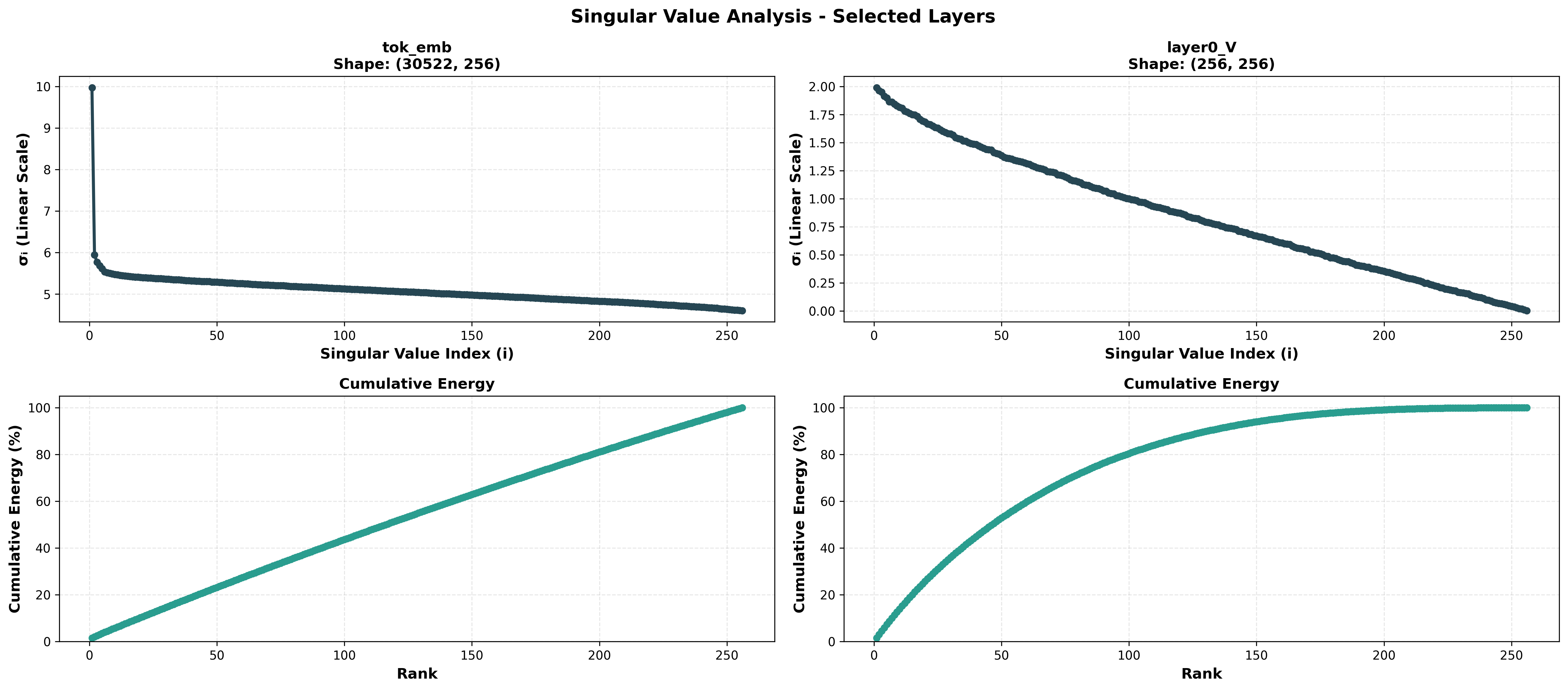
But modern weight matrices often have fast spectral decay.

What Existing Low-Rank Methods Miss

Not LoRA — a different posterior object.

Approach

Backbone

Posterior object

Support of posterior

Post-hoc noise

Pretrained

Noise on fixed W

Full ambient ℝ^mn

Low-rank covariance

Full W means

Covariance approx.

Full ambient ℝ^mn

Bayesian LoRA

Pretrained adapter

Adapter uncertainty

Rank-r adapter only

SBNN (ours)

From scratch

Singular q_W

Rank-r manifold ℳ_r

The differentiator is the support: SBNN puts probability on the rank-r manifold itself, not on ambient ℝ^mn.

The Move

Learn uncertainty in factor space, then map it into weight space.

B^T

Variational posteriorq(A,B)=q_A(A)q_B(B), mean-field Gaussians over factor entries.

Parameter countO(mn) becomes O(r(m+n)); rank controls expressiveness.

Drop-in layersImplemented for dense layers, LSTM gates, and Transformer components.

Pushforward Posterior

The posterior over W is induced, not independently assigned.

q(A,B)factor posterior

T(A,B)=AB^T →

q_Winduced weight posterior

This is the formal turn: the Bayesian object is a pushforward measure on weight space.

Central Theorem

q_W is singular with respect to Lebesgue measure.

If r < min(m,n), and W = AB^T with A ∈ ℝ^m×r, B ∈ ℝ^n×r:

q_W(ℛ_r) = 1 and λ(ℛ_r) = 0 therefore q_W ⟂ λ

The posterior cannot be represented as a full-dimensional density over ℝ^m×n. It lives on zero-volume rank-r support.

Geometric Distinction

Mean-field fills volume. Low-rank mass lives on a manifold.

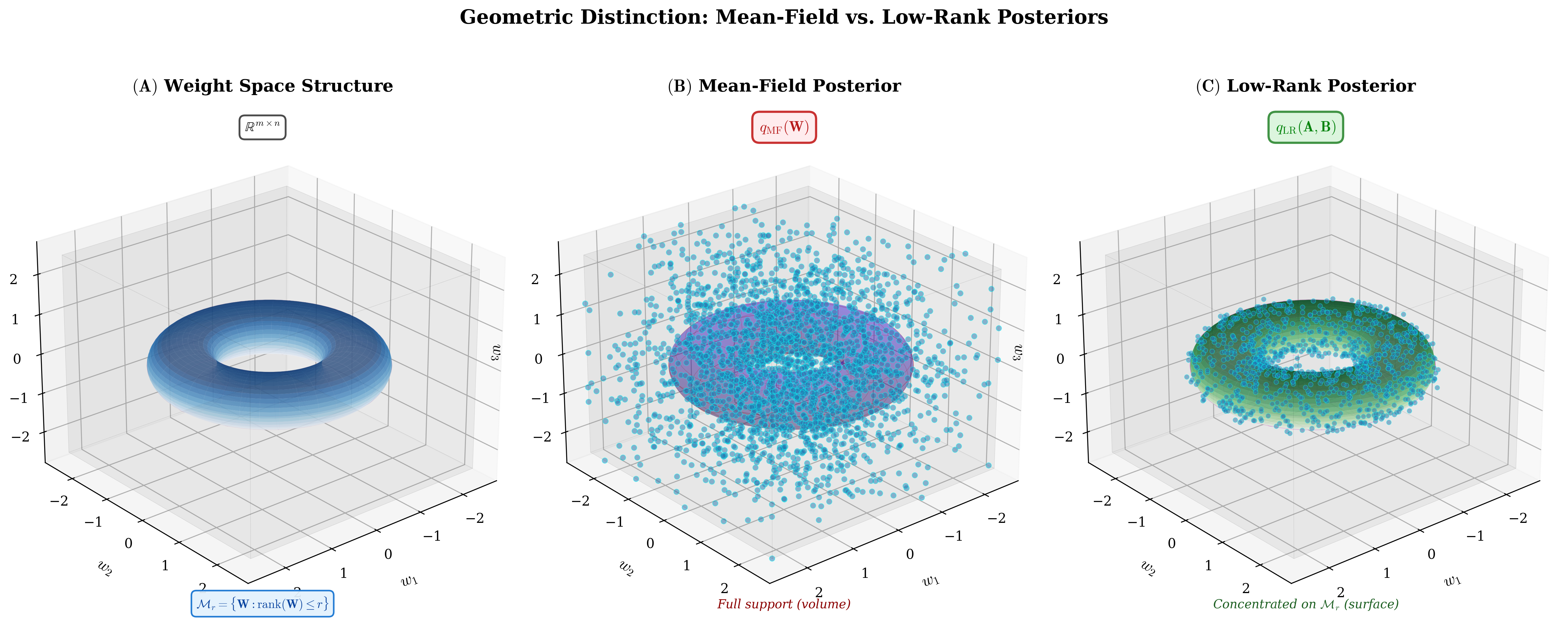
This is why "singular BNN" is the right phrase: the posterior support itself has changed.

Structured Latent-Factor Uncertainty

Mean-field factors do not imply mean-field weights.

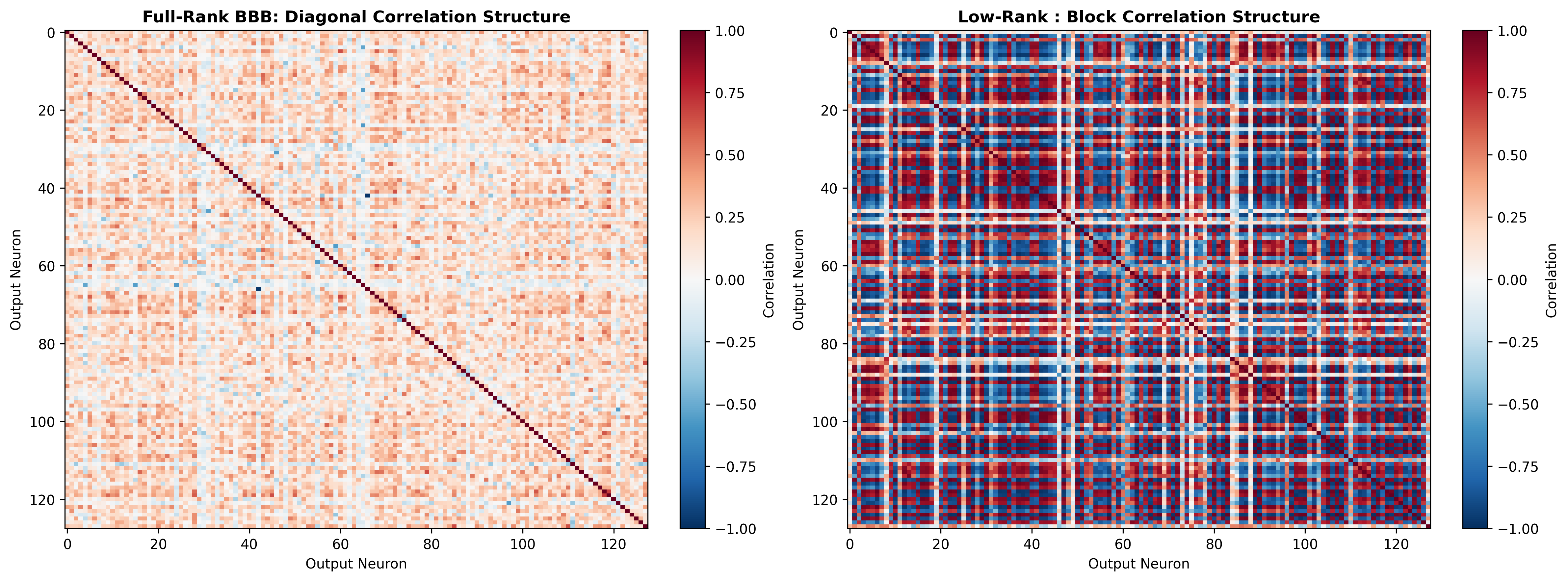
Covariance lemmaEven when A and B have independent entries, W_ij and W_i′j′ can be correlated through shared latent dimensions.

Inductive biasThe model trades independence bias for correlation bias: row/column-level uncertainty propagates coherently.

Rank r controls how expressive these correlations can be.

Theory Stack

The paper gives three theory certificates, not one.

ApproximationEckart–Young–Mirsky controls rank-r approximation by the tail singular values of W*.

Learned factorsError decomposes into learning error ‖W−W_r*‖_F plus unavoidable rank bias σ_>r.

GeneralizationPAC-Bayes complexity scales as √r(m+n), and Gaussian complexity transfers to Bayesian predictive means.

PAC-Bayes and Gaussian complexity bounds

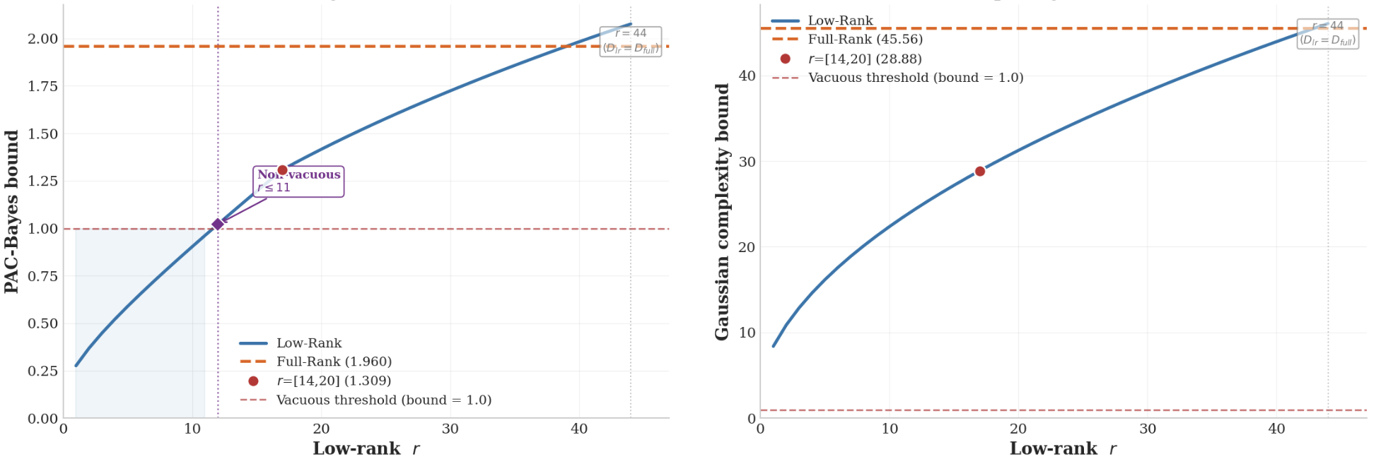
Figure result: PAC-Bayes shows a critical rank transition; Gaussian complexity decreases with rank reduction.

Three Certificates — Formal Statements

Each certificate addresses a distinct aspect of the low-rank posterior.

①

Loss Approximation (Eckart–Young–Mirsky)

|𝔼[ℓ(W*x,y)] − 𝔼[ℓ(W*ᵣx,y)]| ≤ L·R·√(Σᵢ₌ᵣ₊₁ σᵢ²(W*))

Rapid singular-value decay ⇒ small rank-induced bias.

②

PAC-Bayes Generalization Bounds

Complexity(Q_LR)/Complexity(Q_full) ≈ √(r(1/m + 1/n)) ≪ 1 O(r(m+n)) vs O(mn) — tighter bounds when r ≪ min(m,n).

Non-vacuous for low ranks where full-rank BNNs already fail.

③

Gaussian Complexity Transfer

𝒢(F^BNN) ≤ 𝒢(F^{Pinto(C,r)}) f_BNN ∈ conv̄(supp q_W) GC invariant under closure + conv hull

Deterministic rank-sensitive bounds transfer to Bayesian predictive means without degradation.

PAC-Bayes: Complexity Reduction in Detail

Low-rank changes the dominant scaling term in the generalization bound.

Full-Rank MFVI

L(Q) ≤ L̂(Q) + √((C·mn + log(2√N/δ)) / 2N)

Complexity: O(mn)

Low-Rank (Ours)

L(Q) ≤ L̂(Q) + √((C·r(m+n) + log(2√N/δ)) / 2N)

Complexity: O(r(m+n))

Practical numbers for m = n = 512 (relative complexity, lower is better):

25×fewer at r = 64

64×fewer at r = 16

128×fewer at r = 8

Even if empirical risk is slightly higher, the overall bound can still be tighter due to the reduced complexity term.

Implementation

The framework is not architecture-specific.

MLPstandard dense layers
W_ℓ = A_ℓB_ℓ^T

LSTMinput-to-hidden + hidden-to-hidden
factors sampled once per batch

Transformerposition-wise factorization
rank r=16 in SST-2 experiments

Drop-in variational layers make the geometry portable across model families.

Experimental Design

Three architectures. Three data regimes. Six uncertainty baselines.

Dataset

Architecture

Shift

Rank

MIMIC-III ICU mortality

2-layer MLP

adult ICU → newborn ICU

r=15

Beijing PM₂.₅ forecasting

2-layer LSTM

Beijing → Guangzhou

r=14/20

SST-2 sentiment

4-layer Transformer

movie reviews → AGNews

r=16

Baselines: deterministic, Deep Ensemble, Full-Rank BBB, Low-Rank random init, Low-Rank SVD init, Rank-1 multiplicative; SWAG added as supplementary comparator.

Result: MIMIC-III

On clinical shift, low-rank gives the strongest OOD uncertainty.

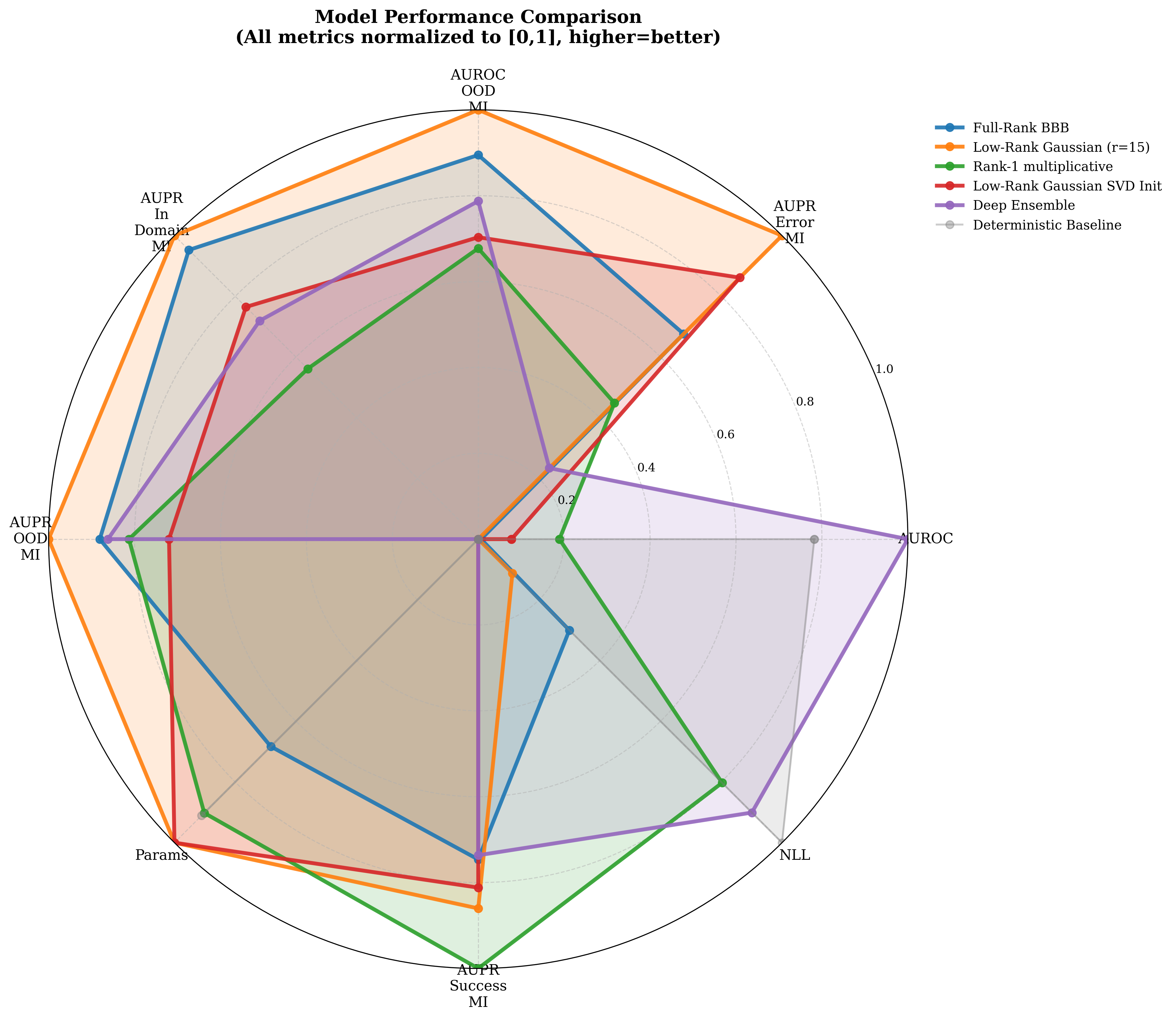
0.802AUC-OOD, best overall

0.788AUPR-OOD, best overall

0.824AUPR-In, best overall

NuanceDeep Ensemble keeps stronger in-domain AUROC and NLL. Low-rank prioritizes epistemic separation under shift.

Parameter reduction: 70% fewer than Full-Rank BBB; 88% fewer than Deep Ensemble.

MIMIC-III · ICU Mortality Prediction (MLP)

Full results — averaged over 5 independent runs.

Model	AUROC ↑	AUPR-Err ↑	AUC-OOD ↑	AUPR-OOD ↑	AUPR-In ↑	NLL ↓	Params ↓
Deterministic	.922	.145	.500	.544	.456	.284	22.4K
Deep Ensemble	.929	.237	.738	.754	.721	.300	112K
Full-Rank BBB	.895	.412	.770	.759	.807	.401	44.8K
★ Low-Rank (ours)	.895	.540	.802	.788	.824	.433	13.6K

70%fewer params than
Full-Rank BBB

88%fewer params than
Deep Ensemble

0.540AUPR-Error
(best in class)

0.802AUC-OOD
(best in class)

Result: Beijing PM₂.₅

For time-series forecasting, uncertainty quality shows up in coverage and abstention.

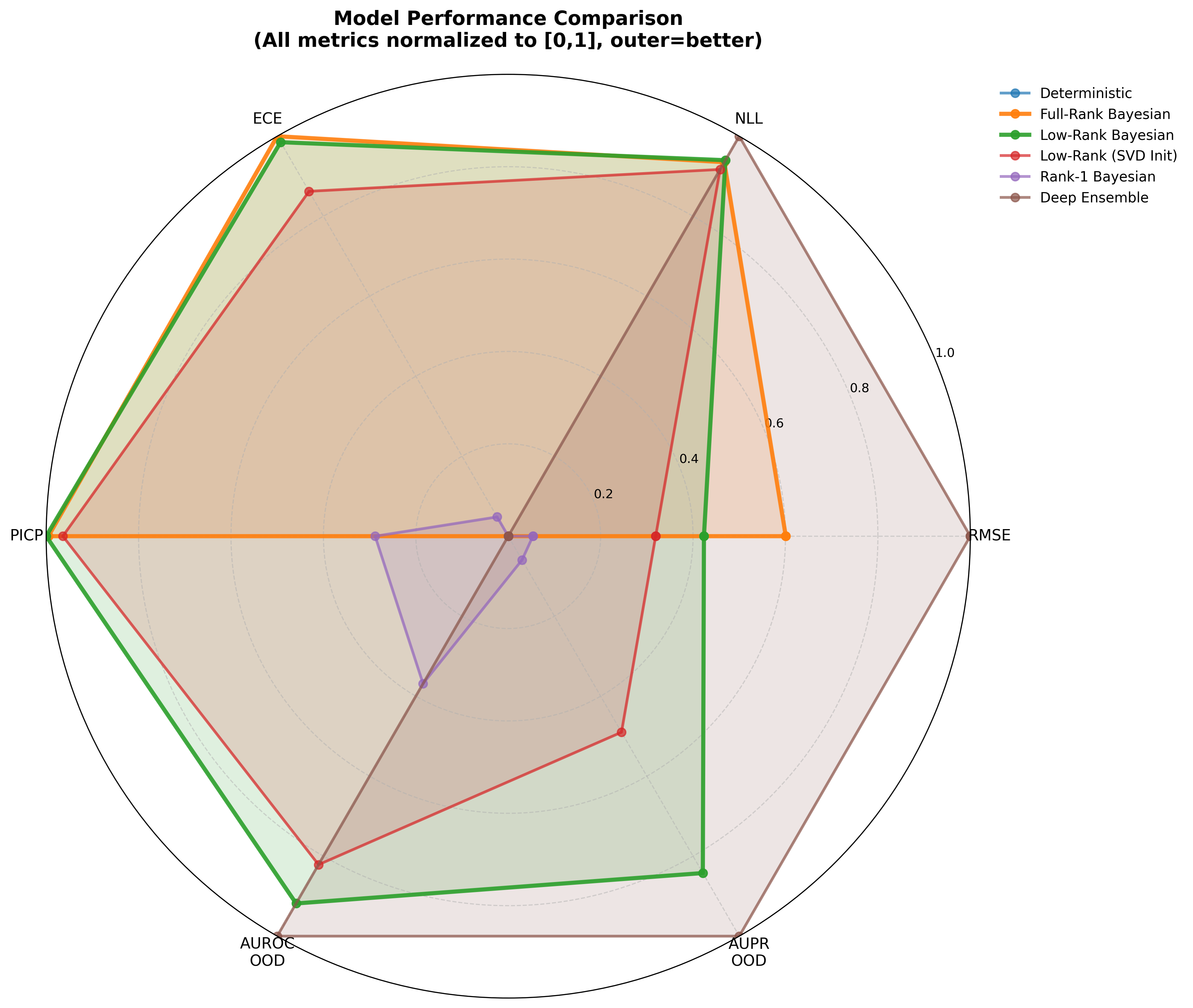
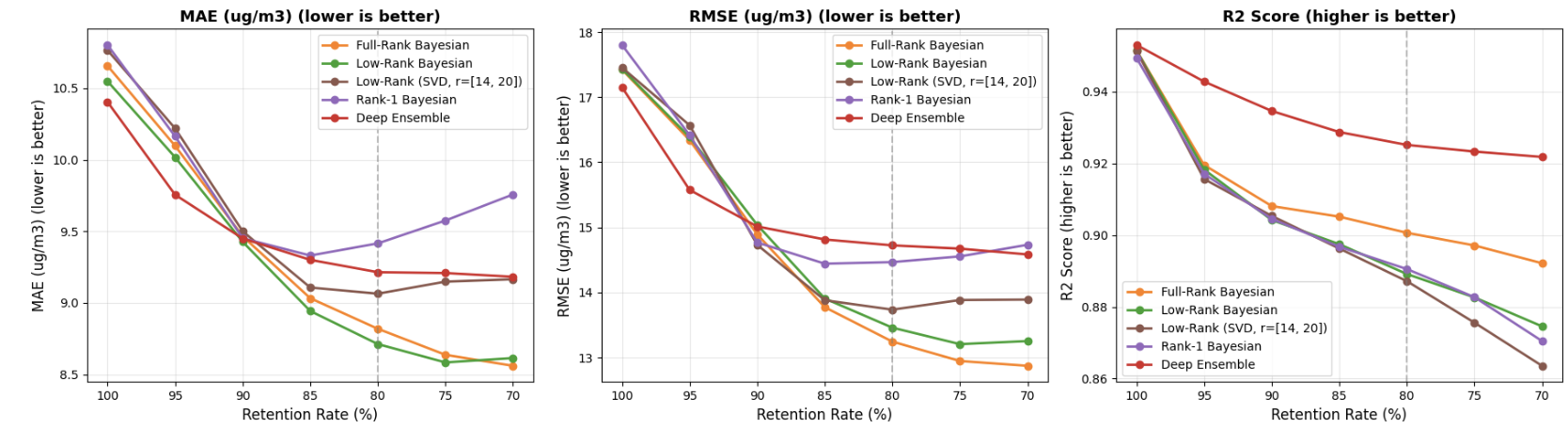
0.790PICP, best coverage

17.4%MAE reduction at 80% retention

64%fewer params than Full-Rank BBB

Beijing PM₂.₅ · Time-Series Forecasting (LSTM)

Full results — averaged over 4 independent runs.

Model	MAE ↓	ECE ↓	PICP ↑	AUROC-OOD ↑	AUPR-OOD ↑	Params ↓
Deterministic	10.79	—	—	.500	.500	33K
Full-Rank BBB	10.55	.111	.788	.492	.743	132K
★ Low-Rank (ours)	10.63	.114	.790	.710	.861	47K
Rank-1 Mult.	10.80	.307	.449	.580	.751	66K
Deep Ensemble	10.45	.317	.310	.730	.883	330K

0.790PICP, best
prediction coverage

17.4%MAE reduction
at 80% retention

6.6×fewer params than
Deep Ensemble

Low-Rank achieves MAE 8.71 vs 9.21 for Deep Ensemble at 80% retention — structured rank-r correlations yield better-calibrated abstention when filtering the 20% most uncertain predictions.

Result: SST-2 Transformer

At Transformer scale, the parameter story becomes decisive.

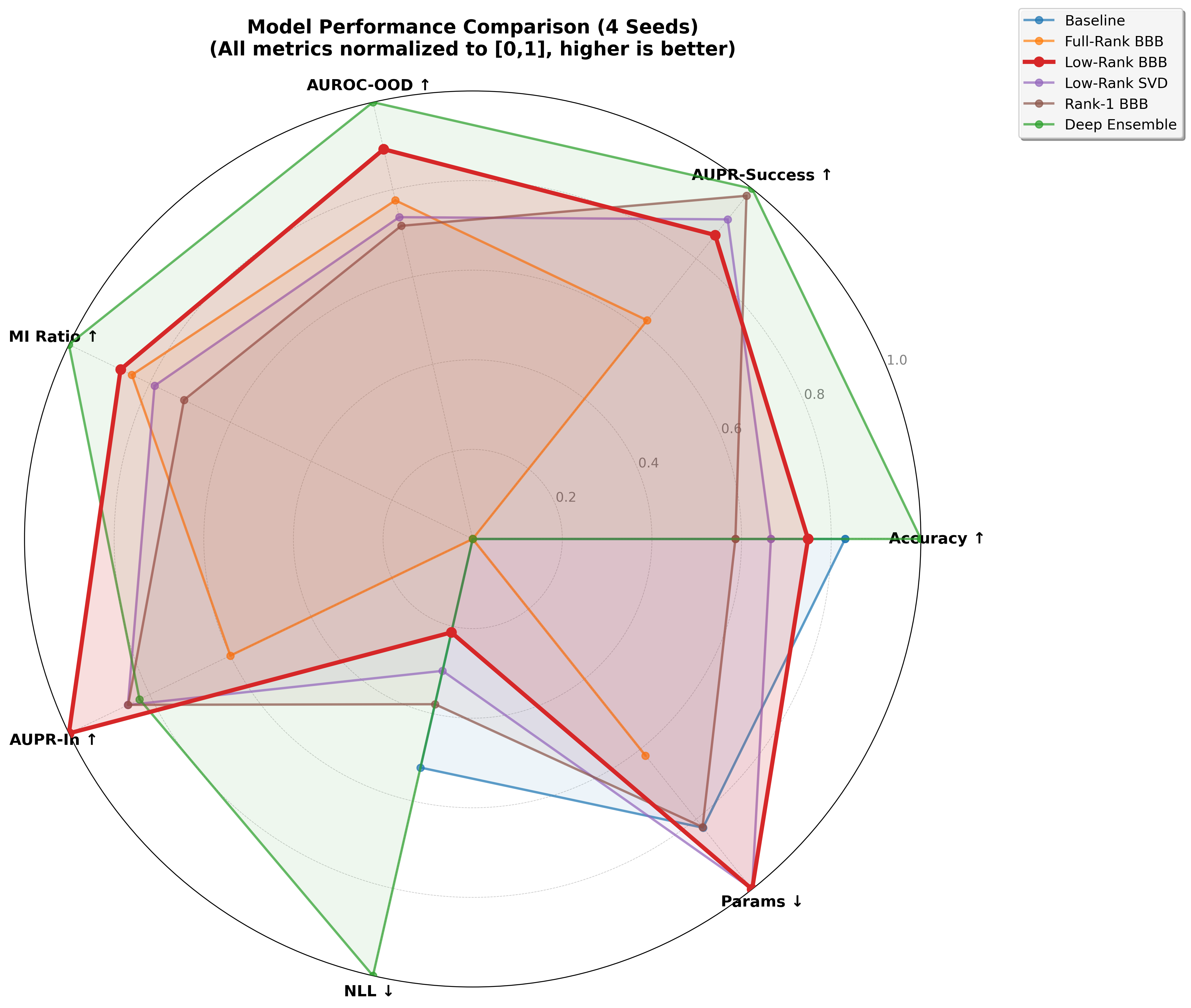
1.5MLow-Rank BBB parameters

13×fewer than Full-Rank BBB

33×fewer than Deep Ensemble

Performance profileLow-Rank BBB: 0.806 accuracy, best AUPR-In, second-best AUROC-OOD. Deep Ensemble remains strongest overall but costs 49.6M parameters.

Training timeLow-Rank trains in 8.2 min vs 23.1 for Full-Rank BBB and 64.7 for Deep Ensemble.

SST-2 Sentiment · Transformer Efficiency

Full results + controlled GPU profiling — averaged over 4 runs.

Model	Acc ↑	NLL ↓	AUROC-OOD ↑	MI Ratio ↑	AUPR-In ↑	Params ↓	Time
Deterministic	.812	.490	.500	.00	.102	9.9M	7.7 min
Deep Ensemble	.825	.434	.657	1.55	.267	49.6M	64.7 min
Full-Rank BBB	.752	.552	.622	1.31	.222	19.8M	23.1 min
★ Low-Rank (ours)	.806	.527	.640	1.35	.302	1.5M	8.2 min

⚡ Controlled GPU Profiling — same device, fixed steps (SST-2)

Model	Params	Peak Memory	Epoch Time
★ Low-Rank BBB (ours)	1.47 M	357.5 MB	5.88 s
Full-Rank BBB	19.84 M	721.1 MB	6.45 s
Deep Ensemble	49.61 M	670.1 MB	18.99 s

Efficiency Evidence

The quality-efficiency frontier changes.

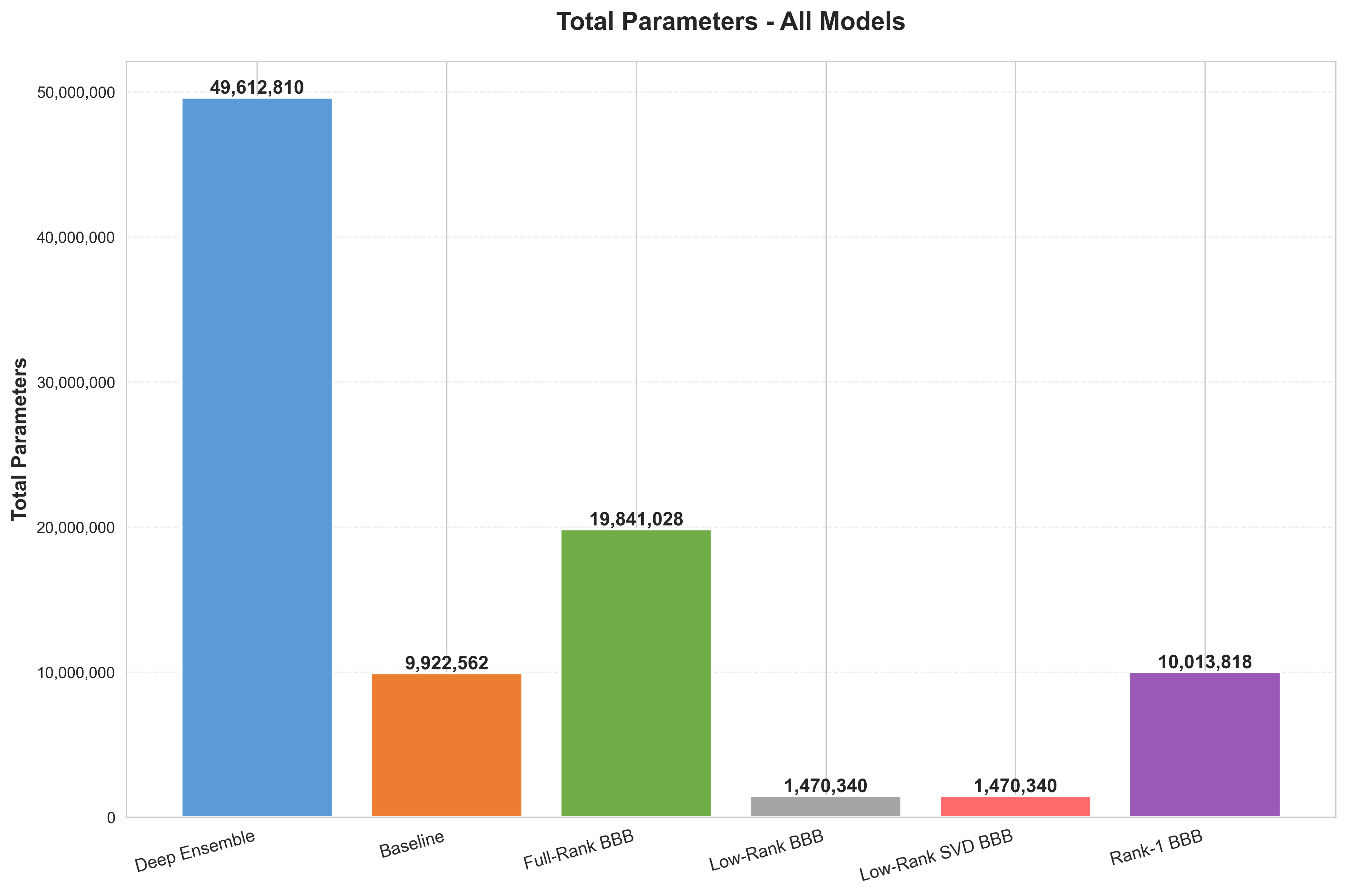
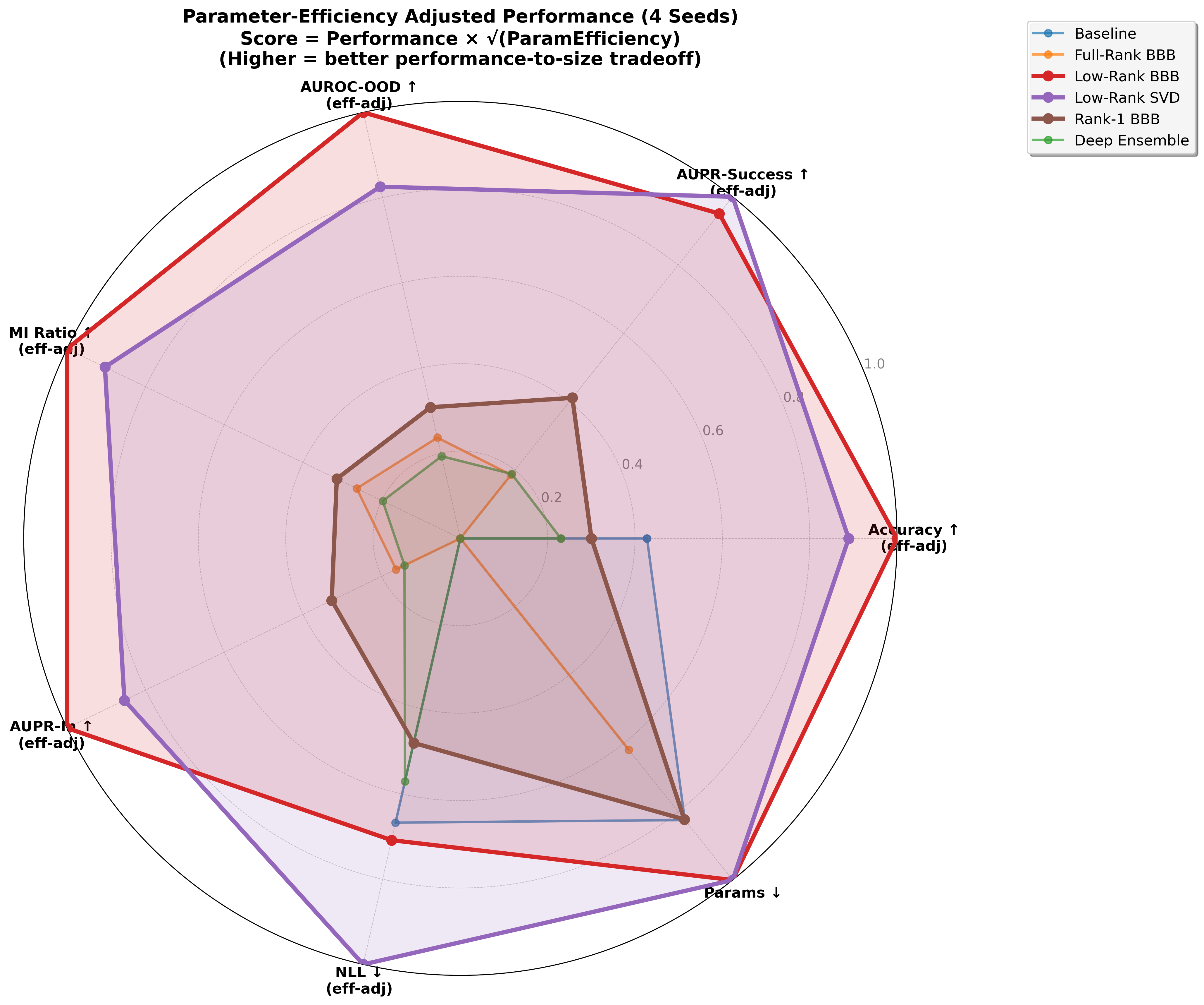
The result is not "low-rank always wins every metric"; it is that useful Bayesian uncertainty becomes plausible at modern parameter scales.

Why Rank Is Plausible

Observed singular value decay supports the rank-r constraint.

When layer spectra decay quickly, the manifold is not an arbitrary bottleneck. It is a structured approximation class.

Theory connectionEYM tail singular values determine rank approximation error; rank ablations and spectra guide practical rank selection.

Comparator: SWAG

A strong posterior baseline does not overturn the central tradeoff.

Setting

SWAG strength

Low-rank advantage

SST-2

Accuracy tied at 0.808 vs 0.806

Better NLL/OOD; 1.47M params vs 208.37M

MIMIC

Higher in-domain AUROC/NLL

OOD MI metrics: 0.802 / 0.788 vs 0.634 / 0.680

Beijing

Higher coverage

Much narrower/costlier tradeoff; stronger OOD for low-rank

SWAG is a credible baseline. However, SBNN's geometry gives a better quality-efficiency path in the paper's target regimes.

Key Insight: Calibration – OOD Detection Tradeoff

A consistent but task-dependent pattern across all three experiments.

MIMIC-III

Low-rank improves OOD detection despite weaker NLL than Deep Ensembles. Structured uncertainty outperforms under clinical domain shift.

SST-2

Deep Ensemble stronger on both NLL and OOD. Low-rank competitive at 33× fewer parameters — a completely different efficiency regime.

Beijing PM₂.₅

Low-rank achieves best calibration, coverage, and selective prediction. OOD advantage is secondary to interval quality.

Hypothesis: The rank constraint on ℛ_r enforces structured weight correlations (Lemma 3.2) that maintain broader epistemic uncertainty. This benefits abstention, coverage, and OOD awareness at the cost of predictive sharpness (NLL). The tradeoff is task-dependent.

✦ Ensembling closes the gap — 5 low-rank members, still cheaper than one full-rank BBB

+0.093AUROC-OOD
0.638 → 0.731

−0.112ECE ↓
0.166 → 0.054

−0.108NLL ↓
0.523 → 0.415

Honest Takeaway

The empirical message is not compression alone.

Where low-rank shinesOOD separation on MIMIC; coverage/selective prediction on Beijing; efficiency-adjusted uncertainty on SST-2.

Where ensembles remain strongIn-distribution likelihood and sharpness can favor Deep Ensembles; calibration gaps remain in some settings.

Why that mattersTrustworthy AI often needs useful uncertainty under shift, abstention, and deployment constraints, not only marginal NLL.

SBNNs make that goal more practical: structured uncertainty, lower cost, and scalable to modern architectures.

Research Agenda

A platform for scalable Bayesian posteriors in modern architectures.

Adaptive rank selectionRanks chosen by spectra, validation tradeoffs, or sparse priors rather than fixed grids.

Bayesian TransformersStructured uncertainty for large sequence models without ensemble-scale cost.

Beyond Gaussian factorsLaplace, spike-and-slab, and richer factor distributions while keeping singular support.

Trustworthy AIUncertainty that supports abstention, coverage, OOD awareness, and constrained deployment.

Closing

Singular posterior geometry for scalable Bayesian deep learning.

Singular Bayesian Neural Networks

arradiat.github.io/projects/singular-bnn arxiv.org/abs/2602.00387 github.com/arradiat/SBNN mame.toure@mail.mcgill.ca

SingularBayesian NeuralNetworks