ICML 2026

Singular Bayesian
Neural Networks

Low-rank Bayesian neural networks with singular posterior geometry, reduced complexity scaling, and scalable uncertainty quantification.

Mame Diarra Touré, David A. Stephens
McGill University
$W = AB^\top$
Low-rank Bayesian posteriors concentrate on rank-constrained manifolds.
TL;DR

We parameterize Bayesian neural network weights through low-rank factors $W = AB^\top$, inducing a singular posterior geometry concentrated on the rank-$r$ manifold. This reduces variational complexity from $O(mn)$ to $O(r(m+n))$ while maintaining competitive uncertainty-aware performance across MLPs, LSTMs, and Transformers.

01

What this paper shows

Low-rank variational BNNs do not merely save parameters — they change the geometry, covariance structure, and complexity of the posterior.

Method

End-to-end variational learning over low-rank factors $W = AB^\top$, trained from scratch without pretrained backbones.

Geometry

The induced posterior $q_W$ is a pushforward measure supported on the rank-$r$ manifold $\mathcal{R}_r \subset \mathbb{R}^{m \times n}$.

Singularity

$q_W$ is singular with respect to Lebesgue measure on the ambient weight space.

Correlations

Mean-field factors over $A, B$ still induce structured, non-trivial covariance between entries of $W$ through shared latent dimensions.

Theory

Three certificates: approximation error (Eckart–Young–Mirsky), PAC-Bayes generalization bounds, and Gaussian complexity transfer.

Evidence

Validated on MLPs (MIMIC-III), LSTMs (Beijing PM₂.₅), and Transformers (SST-2) with OOD evaluation on domain-shifted test sets.

Core thesis: low-rank is not merely parameter economy — it changes posterior support, covariance, and capacity.
02

Motivation

Bayesian neural networks provide principled uncertainty, but full weight-space inference does not scale. Three obstacles block practical deployment.

O(mn)

Parameter explosion

Standard mean-field MFVI requires 2 variational parameters per weight, doubling the parameter count per layer, scaling as $O(mn)$ for a single matrix.

Independence assumption

Fully factorized posteriors ignore structured correlations between weights, limiting expressiveness and the model's ability to represent epistemic uncertainty coherently.

Ensemble cost

Deep Ensembles, the practical gold standard, require 5 full model copies, making them prohibitively expensive for modern-scale architectures.

Key gap: No prior work trains low-rank BNNs end-to-end across diverse architectures (MLPs, LSTMs, Transformers) with rigorous theoretical guarantees on posterior geometry.

What existing low-rank methods miss

This paper is not LoRA with uncertainty pasted on top. The novelty is the induced posterior measure over $W$: its support, geometry, covariance, and complexity all change.

Post-hoc perturbations Pretrained backbone · noise added around fixed deterministic weights
Not end-to-end uncertainty
Low-rank posterior covariance Full $W$ means still $O(mn)$ · low rank only in the covariance approximation
Still O(mn) weight means
Bayesian LoRA Pretrained / fine-tuning · adapter uncertainty only · affine subspace support
Not from-scratch BNN training
★ SBNN (ours) Learned from scratch · singular $q_W$ concentrated on rank-$r$ manifold · structured covariance via shared factors
Pushforward posterior
03

Core idea

From mean-field to structured low-rank geometry

Standard Bayesian neural networks often rely on fully factorized posteriors that ignore structured correlations between weights. We instead introduce low-rank variational factors:

$$A \in \mathbb{R}^{m \times r}, \qquad B \in \mathbb{R}^{n \times r}, \qquad W = AB^\top.$$

Although the factors themselves can be mean-field, the induced posterior over $W$ becomes highly structured, introducing correlations through shared latent factors. Optimized via the reparameterization trick (Bayes by Backprop) with Adam — implemented as drop-in Keras layer replacements for dense layers, LSTM gates, and Transformer projections.

Complexity $O(r(m+n))$ instead of $O(mn)$
Posterior support rank-$r$ manifold singular in ambient matrix space
Architectures MLP · LSTM · Transformer drop-in Bayesian layers

Evidence Lower Bound (ELBO)

$$\mathcal{L}(q) \;=\; \underbrace{\mathbb{E}_{q_A q_B}\!\left[\log p(\mathcal{D}\mid AB^\top)\right]}_{\text{Data fit}} \;-\; \underbrace{\beta\,\mathrm{KL}(q_A \,\|\, p_A)}_{\text{Reg. on }A} \;-\; \underbrace{\beta\,\mathrm{KL}(q_B \,\|\, p_B)}_{\text{Reg. on }B}$$
Data fit Expected log-likelihood under the joint factor posterior
Regularisation on A KL divergence from prior on left factor
Regularisation on B KL divergence from prior on right factor
Key insight: Because $q(A,B) = q_A(A)\,q_B(B)$ factorizes, the KL term splits into two independent pieces — one over $A$, one over $B$ — enabling efficient parallel computation. All three terms in the ELBO are estimated via Monte Carlo: sample $\varepsilon_A, \varepsilon_B \sim \mathcal{N}(0,I)$, form $A = \mu_A + \sigma_A \circ \varepsilon_A$ and $B = \mu_B + \sigma_B \circ \varepsilon_B$, compute $W = AB^\top$, and backpropagate through the reparameterization.
Scale mixture prior
$$p_A(A) = \prod_j \!\left[{\tfrac{1}{2}}\mathcal{N}(a_j\!\mid\!0,1) + {\tfrac{1}{2}}\mathcal{N}(a_j\!\mid\!0,e^{-6})\right]$$

A broad Gaussian ($\sigma_1^2=1$) and a narrow spike ($\sigma_2^2 \approx 0.002$): encourages sparse structure while allowing occasional large weights. Same prior for $B$.

Reparameterization (Bayes by Backprop)
$$\sigma = \log(1+e^\rho),\quad A = \mu_A + \sigma_A \circ \varepsilon_A,\quad \varepsilon_A \sim \mathcal{N}(0,I)$$

Positivity enforced via softplus. Sampling is differentiable w.r.t. $(\mu_A,\rho_A)$, allowing gradients to flow through Monte Carlo ELBO estimates.

Architecture implementations

Each architecture requires one key adaptation. The variational layers are drop-in replacements for standard Keras layers.

MLP

Per-layer factorization

Each dense layer $W_\ell \in \mathbb{R}^{d_\ell \times d_{\ell+1}}$ uses $W_\ell = A_\ell B_\ell^\top$ with its own rank $r_\ell$, tunable independently. No architecture-specific modifications needed — identical variational layers.

W_ℓ = A_ℓ Bℓᵀ · each layer has own rℓ
LSTM

Weight caching across time steps

$W_{ih}$ and $W_{hh}$ are factorized. Following Fortunato et al. (2017), factors $A,B$ are sampled once per batch, $W = AB^\top$ is cached across all $T$ time steps, and KL divergence is computed once per sequence. Forget gate bias initialized to 1.0.

sample once → cache W=ABᵀ → reuse t=1…T → new batch
Transformer

Embedding sparsity trick

Q/K/V/FF projections use the same variational layers as MLPs. For the embedding $W_{emb} \in \mathbb{R}^{V \times d}$, only rows of $A$ corresponding to tokens in the current batch are sampled, reducing cost from $O(Vd)$ to $O(|U|r + dr)$ where $|U|$ is unique tokens.

O(Vd) → O(|U|r + dr) · independent factors per head
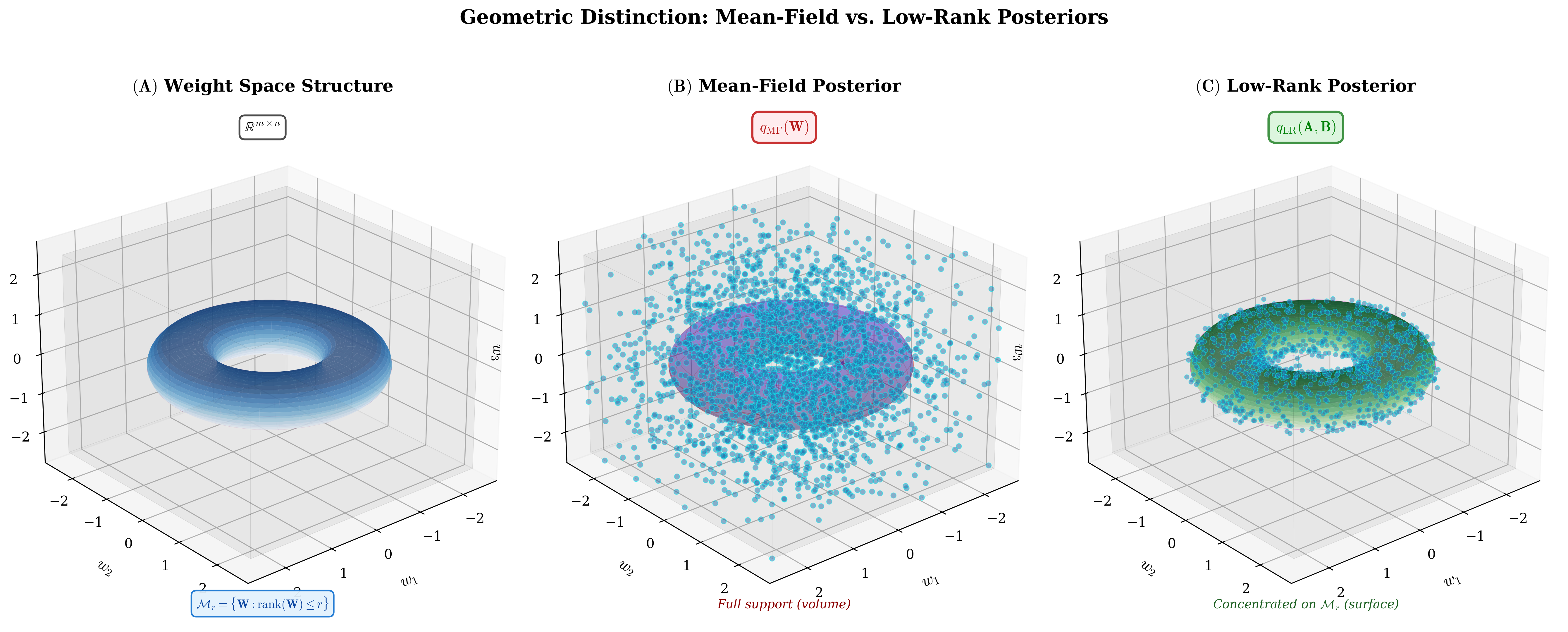
Posterior geometry figure
Posterior geometry. Mean-field posteriors occupy a full-dimensional volume, whereas low-rank posteriors concentrate on the rank-constrained manifold.

GPU Profiling · SST-2 · Controlled single-device benchmark

Orders of magnitude more efficient — without sacrificing uncertainty quality.

All models trained for the same number of steps on the same GPU.

★ Low-Rank BBB (ours)
Parameters 1.47 M
Peak GPU memory357.5 MB
Epoch time 5.88 s
Full-Rank BBB
Parameters 19.84 M
Peak GPU memory721.1 MB
Epoch time 6.45 s
Deep Ensemble (M=5)
Parameters 49.61 M
Peak GPU memory670.1 MB
Epoch time 18.99 s

Low-Rank BBB: 13× fewer parameters than Full-Rank BBB, ~50% of the peak memory, and 3.2× faster per epoch than Deep Ensemble. Full Bayesian uncertainty at a fraction of the cost.

04

The mathematical mechanism

The paper's key move is to define a simple mean-field posterior in factor space, then study the induced posterior measure over the full weight matrix.

Notation. Throughout, $W^\star \in \mathbb{R}^{m \times n}$ denotes the optimal full-rank weight matrix (i.e. the population-risk minimiser), with singular values $\sigma_1(W^\star) \ge \sigma_2(W^\star) \ge \cdots$. Its best rank-$r$ approximation — given by the truncated SVD — is $W_r^\star = \sum_{i=1}^{r} \sigma_i(W^\star)\, u_i v_i^\top$.

Low-rank Bayesian weight matrix

$$W = AB^\top,\qquad A \in \mathbb{R}^{m \times r},\quad B \in \mathbb{R}^{n \times r}.$$

The variational posterior is placed over the factors rather than directly over every entry of the full matrix.

Factor posterior

$$q(A,B)=q_A(A)q_B(B).$$

The factors may be mean-field, but the induced posterior over $W$ is not an independent posterior over weight entries.

Pushforward posterior

$$q_W = T_{\#}q_{A,B},\qquad T(A,B)=AB^\top.$$

This pushforward measure is the central object: it describes the posterior distribution over the actual weight matrix $W$.

Singular support theorem

$$q_W(\mathcal{R}_r)=1,\qquad \lambda(\mathcal{R}_r)=0,\qquad q_W \perp \lambda.$$

When $r < \min(m,n)$, the posterior is supported on the rank-at-most-$r$ set $\mathcal{R}_r$, which has Lebesgue measure zero in the ambient matrix space.

Rank-induced approximation bias (Eckart–Young–Mirsky)

$$\left| \mathbb{E}[\ell(W^\star x,y)] - \mathbb{E}[\ell(W_r^\star x,y)] \right| \le LR\sqrt{\sum_{i>r}\sigma_i^2(W^\star)}.$$

The loss gap between the optimal full-rank solution $W^\star$ and its best rank-$r$ approximation $W_r^\star$ is controlled by the tail singular values. Rapid spectral decay means small rank-induced bias.

Decomposition of approximation error (Theorem 3.7)

In practice, the learned $W = AB^\top$ may not achieve the optimal rank-$r$ approximation $W_r^\star$. The total error decomposes into two additive components:

$$\bigl|\ell(Wx,y) - \ell(W^\star x,y)\bigr| \;\le\; LR\!\Bigl(\underbrace{\|W - W_r^\star\|_F}_{\text{learning error}} \;+\; \underbrace{\sqrt{\sum_{i>r}\!\sigma_i^2(W^\star)}}_{\text{rank bias}}\Bigr).$$
Learning error ‖W − W_r*‖_F

How far the trained factorization is from the optimal rank-$r$ solution. Reducible with better optimization — not a fundamental limitation.

Rank bias √(Σ σᵢ²(W*))

The unavoidable error from restricting to rank $r$. Small when layer spectra decay quickly — which modern networks exhibit.

Structured covariance

$$\mathrm{Cov}(W_{ij},W_{i'j'}) = \sum_k \Big[ \mathbb{E}[A_{ik}A_{i'k}] \mathbb{E}[B_{jk}B_{j'k}] - \mathbb{E}[A_{ik}]\mathbb{E}[A_{i'k}] \mathbb{E}[B_{jk}]\mathbb{E}[B_{j'k}] \Big].$$

Shared latent factors induce non-zero covariance between weight entries, even though the factor posterior itself is mean-field. Rank $r$ controls how expressive these correlations can be.

Row correlation
When $i = i'$ (same row), weights are correlated through the shared $A$ factor rows — updating one connection perturbs the whole row.
Column correlation
When $j = j'$ (same column), weights are correlated through the shared $B$ factor rows — propagating uncertainty column-wise.
Rank-modulated coupling
All $r$ latent dimensions contribute to correlation strength — higher rank allows richer correlation patterns.
05

Theory

The paper provides three theory certificates. Each addresses a distinct aspect of the low-rank posterior's behaviour.

① Loss Approximation

$$q_W(\mathcal{R}_r)=1,\quad \lambda(\mathcal{R}_r)=0,\quad q_W \perp \lambda.$$

The induced posterior is singular w.r.t. Lebesgue measure on the ambient weight space.

② PAC-Bayes Generalization

$$\sqrt{\frac{r(m+n)}{mn}}$$

Low-rank posteriors reduce the dominant complexity scaling term when $r \ll \min(m,n)$.

③ Gaussian Complexity Transfer

$$\mathcal{G}(F^\mathrm{BNN}) \;\le\; \mathcal{G}(F^{\mathrm{Pinto}(C,r)})$$

The BNN predictive mean lies in the closed convex hull of the support class. Gaussian complexity is invariant under convex hull and closure, so deterministic complexity bounds transfer to Bayesian predictive means.

Three guarantees in detail

Loss Approximation (Eckart–Young–Mirsky)

$$\bigl|\mathbb{E}[\ell(W^\star x,y)] - \mathbb{E}[\ell(W_r^\star x,y)]\bigr| \le LR\!\sqrt{\textstyle\sum_{i>r}\sigma_i^2(W^\star)}$$

The loss gap between the optimal full-rank $W^\star$ and its best rank-$r$ approximation $W_r^\star$ (both defined in §04) is controlled by the tail singular values. Rapid spectral decay means small rank-induced bias.

PAC-Bayes Generalization Bounds

$$L(Q) \le \hat{L}(Q) + \sqrt{\frac{C_{\max}\cdot r(m+n) + \log(2\sqrt{N}/\delta)}{2N}}$$

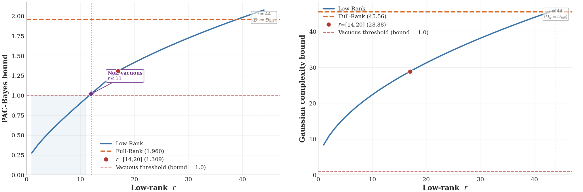
Full-rank MFVI complexity scales as $O(mn)$; low-rank scales as $O(r(m+n))$. The ratio $\mathrm{Complexity}(Q_\mathrm{LR})/\mathrm{Complexity}(Q_\mathrm{full}) \approx \sqrt{r(1/m + 1/n)} \ll 1$ when $r \ll \min(m,n)$. The bound is non-vacuous for low ranks where full-rank BNNs already fail.

Gaussian Complexity Transfer

$$\mathcal{G}(F^\mathrm{BNN}) \;\le\; \mathcal{G}(F^{\mathrm{Pinto}(C,r)})$$

The BNN predictive mean lies in $\overline{\mathrm{conv}}(\mathrm{supp}\,q_W)$. Since Gaussian complexity is invariant under convex hull and closure, the deterministic low-rank complexity bound $\mathcal{G}(F^{\mathrm{Pinto}(C,r)})$ transfers directly to the Bayesian predictive mean — linking frequentist generalization theory to the Bayesian low-rank posterior.

What singularity means — and why it matters

Standard mean-field posteriors $q(W)=\prod_{ij}\mathcal{N}(w_{ij}|\mu_{ij},\sigma_{ij}^2)$ are absolutely continuous with respect to Lebesgue measure: they have positive density everywhere in $\mathbb{R}^{m\times n}$. Our induced $q_W$ is singular continuous — it has no point masses, yet it cannot be represented by any density function.

Proof intuition: suppose $q_W$ had a density $f$ w.r.t. Lebesgue measure $\lambda$. Then $q_W(\mathcal{R}_r) = \int_{\mathcal{R}_r} f\,d\lambda = 0$ (since $\lambda(\mathcal{R}_r)=0$) — contradicting $q_W(\mathcal{R}_r)=1$. Therefore no such density exists. The posterior concentrates its entire mass on a set of zero volume.

Bias of independence vs. bias of correlation

As argued by Wilson (2020), generalization depends on the support and inductive biases of the posterior. Mean-field and SBNN impose fundamentally different biases.

Mean-field: bias of independence

Treats each weight as a freely adjustable parameter. Updating $w_{ij}$ only touches that entry — local memorization is possible. The posterior has positive density everywhere in $\mathbb{R}^{m\times n}$, imposing no structural constraint on which weight configurations are reached.

SBNN: bias of correlation

Restricts posterior support to $\mathcal{R}_r$. Updating $W_{ij} = \sum_k A_{ik}B_{jk}$ requires modifying shared factors that affect entire rows and columns simultaneously. This prevents local memorization and enforces coherent uncertainty propagation across connected weights.

Gaussian Complexity: capacity control beyond parameter count

Although Gaussian complexity is not the canonical Bayesian tool (PAC-Bayes is), it offers a complementary perspective: low-rank layers impose geometric constraints that reduce complexity beyond what parameter-count arguments capture.

Honest caveat: empirically, the Gaussian complexity bounds are vacuous for both full-rank and low-rank models — they exceed 1 and do not provide practical generalization certificates. What they do formalize is how rank constraints and spectral norms jointly control model capacity, suggesting rank-induced restrictions contribute to the good generalization often observed in practice. The proof is also architecturally transparent: the BNN predictive mean belongs to the closed convex hull of the support class, and Gaussian complexity is invariant under convex hull and closure — so deterministic rank-sensitive bounds transfer to Bayesian predictive means without degradation.

Complexity reduction in practice

For $m=n=512$ (relative complexity vs full-rank MFVI, lower is better):

25×
fewer at r=64
64×
fewer at r=16
128×
fewer at r=8
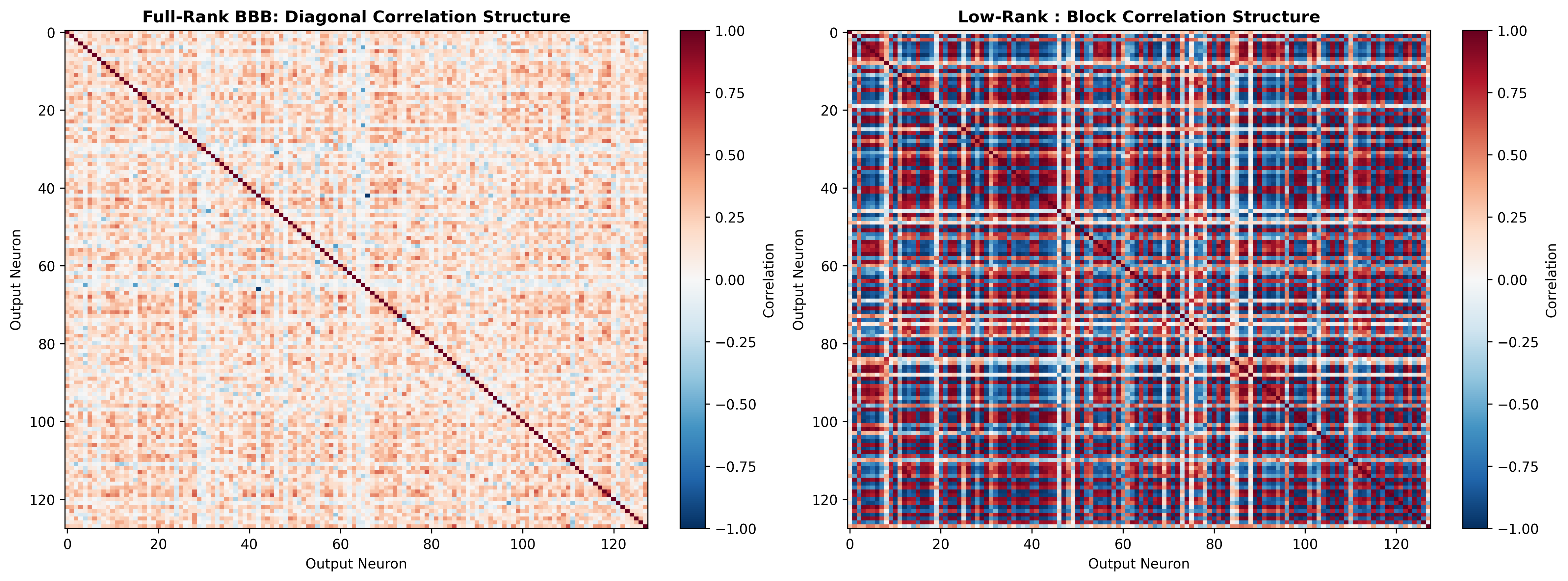
Weight correlation heatmap
Induced correlation structure in low-rank Bayesian weights.
Combined bound figure
PAC-Bayes and Gaussian complexity perspectives on low-rank scaling. Both bounds decrease monotonically as rank drops.
06

Why rank is plausible

The rank-$r$ manifold is not an arbitrary bottleneck — it is a structured approximation class supported by the empirical spectral structure of learned neural network weights.

Observed singular value decay

Weight matrices in trained neural networks routinely exhibit fast singular value decay: a small number of dominant directions captures most of the representational capacity. This motivates the rank-$r$ manifold as a natural approximation class rather than an artificial constraint.

EYM tail bound is tight in practice

The Eckart–Young–Mirsky bound controls rank approximation error through tail singular values $\sigma_{r+1}^2(W^\star) + \cdots$. When layer spectra decay quickly, these tails are small, and the rank-$r$ bias is genuinely negligible.

Rank ablations confirm the effect

Experiments include SVD-initialized vs. randomly initialized low-rank factors, and rank ablations across architectures.

Practical rank selection

Ranks are chosen per-architecture based on empirical validation: $r=15$ for the MLP on MIMIC-III, $r=14/20$ for the LSTM on Beijing PM₂.₅, and $r=16$ for the Transformer on SST-2. Adaptive rank selection via sparse priors is a natural future direction.

Parameter-count intuition

Move the rank slider to compare full-rank and low-rank parameterization for a single $256 \times 256$ layer.

Full rank
65536
Low rank
8192

8× fewer parameters for a 256 × 256 layer.

07

Experimental design

Three architectures. Three domain-shift scenarios. Six uncertainty baselines. Each setting includes OOD evaluation on held-out distribution shifts.

MLP · Clinical

MIMIC-III ICU Mortality

In-dist 40,406 adult ICU patients, 44 clinical features
OOD Adult ICU → Newborn ICU (5,357 samples)
Metrics AUROC · AUC-OOD · AUPR-OOD · AUPR-In · NLL
r = 15
LSTM · Time Series

Beijing PM₂.₅ Forecasting

In-dist 29,213 train samples, 24-hour sliding windows
OOD Beijing → Guangzhou climate (20,050 samples)
Metrics MAE · ECE · PICP · AUROC-OOD · AUPR-OOD
r = 14, 20
Transformer · NLP

SST-2 Sentiment

In-dist 67,349 train, 872 dev (movie reviews)
OOD Movie reviews → AG News (7,600 samples)
Metrics Accuracy · NLL · AUROC-OOD · MI Ratio · Params · Time
r = 16
Baselines: Deterministic · Deep Ensemble (M=5) · Full-Rank BBB · Low-Rank (random init) · Low-Rank (SVD init) · Rank-1 Multiplicative · SWAG (supplementary). All Bayesian models optimized with Adam via the reparameterization trick.
MLP · Clinical Experiment 01 / 03

MIMIC-III ICU Mortality

Adult ICU in-distribution → Newborn ICU out-of-distribution  ·  rank r = 15
ModelAUROC ↑AUPR-Err ↑ AUC-OOD ↑AUPR-OOD ↑AUPR-In ↑ NLL ↓Params ↓
Deterministic.922.145 .500.544.456 .28422.4k
Deep Ensemble.929.237 .738.754.721 .300112k
Full-Rank BBB.895.412 .770.759.807 .40144.8k
Low-Rank BBB.895.540 .802.788.824 .43313.6k

Best OOD detection metrics in the clinical-shift setting, with 70% fewer parameters than Full-Rank BBB.

.802 AUC-OOD
best overall
70% fewer params vs
Full-Rank BBB
88% fewer params vs
Deep Ensemble
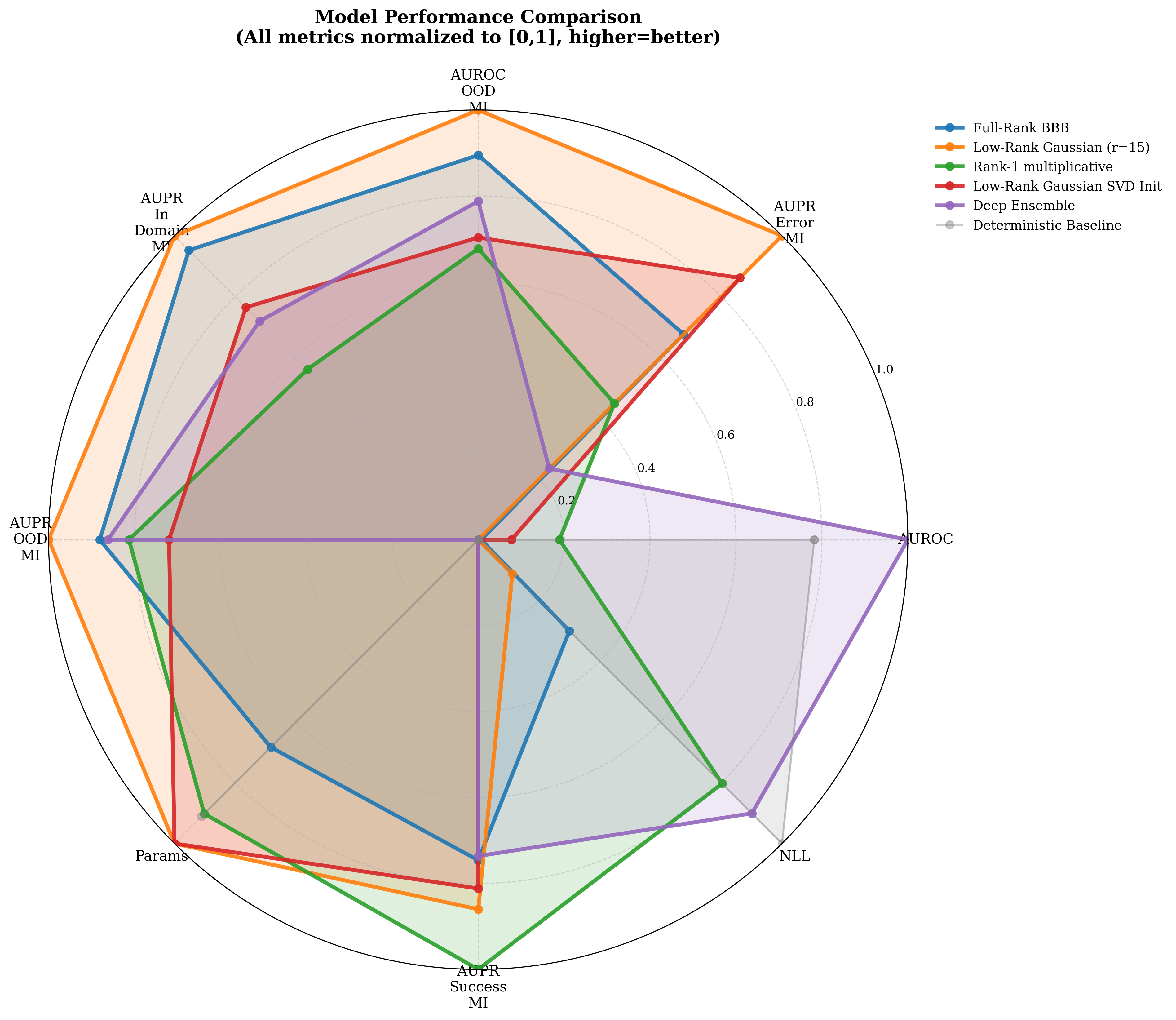
MIMIC-III multi-seed radar

Multi-seed averaged uncertainty metrics — MIMIC-III.

LSTM · Time Series Experiment 02 / 03

Beijing PM₂.₅ Forecasting

Beijing in-distribution → Guangzhou out-of-distribution  ·  ranks r = 14, 20
ModelMAE ↓ECE ↓PICP ↑ AUROC-OOD ↑AUPR-OOD ↑Params ↓
Deterministic10.79 .500.50033K
Full-Rank BBB10.55.111.788 .492.743132K
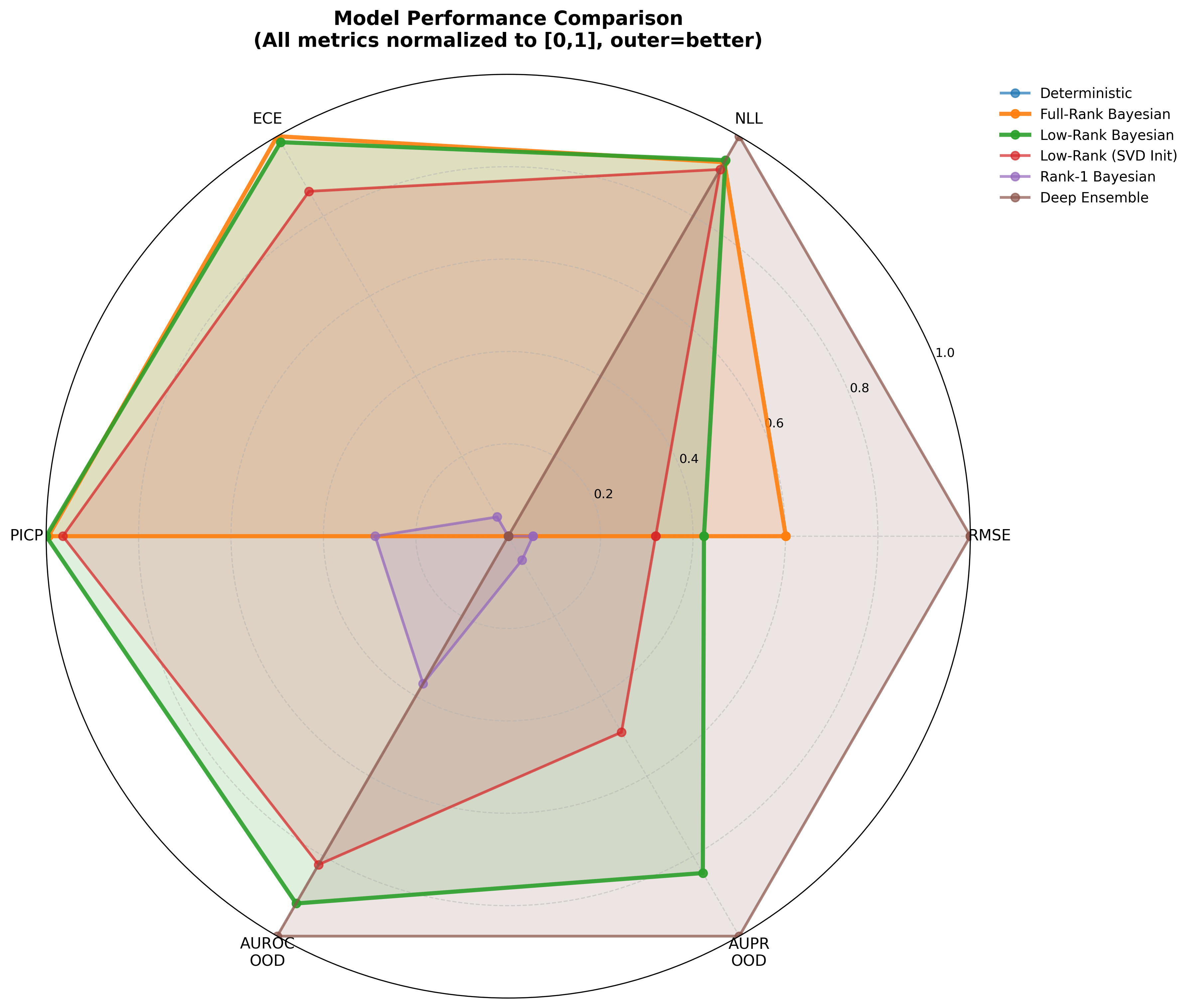
Low-Rank BBB10.63.114.790 .710.86147K
Deep Ensemble10.45.317.310 .730.883330K

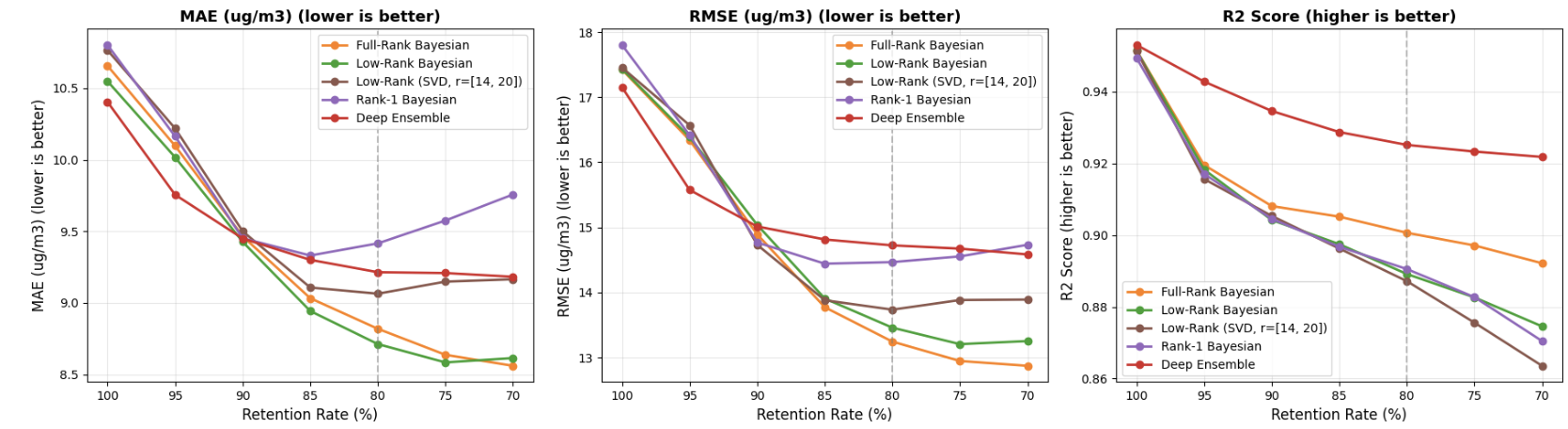
Best coverage (PICP) among Bayesian methods. At 80% retention, Low-Rank BBB achieves MAE 8.71 vs 9.21 for Deep Ensemble — structured correlations improve selective prediction quality.

17.4% MAE reduction
at 80% retention
.790 PICP
best coverage
64% fewer params vs
Full-Rank BBB
Selective prediction curve

Selective prediction: Low-Rank achieves lower MAE at each retention threshold.

LSTM radar

Uncertainty metric radar — LSTM · Beijing PM₂.₅.

Transformer · NLP Experiment 03 / 03

SST-2 Sentiment (Transformer)

Movie reviews in-distribution → AG News out-of-distribution  ·  rank r = 16
ModelAcc ↑NLL ↓ AUROC-OOD ↑MI Ratio ↑AUPR-In ↑ Params ↓Time
Deterministic.812.490 .500.000.102 9.9M7.7 min
Deep Ensemble.825.434 .6571.55.267 49.6M64.7 min
Full-Rank BBB.752.552 .6221.31.222 19.8M23.1 min
Low-Rank BBB.806.527 .6401.35.302 1.5M8.2 min

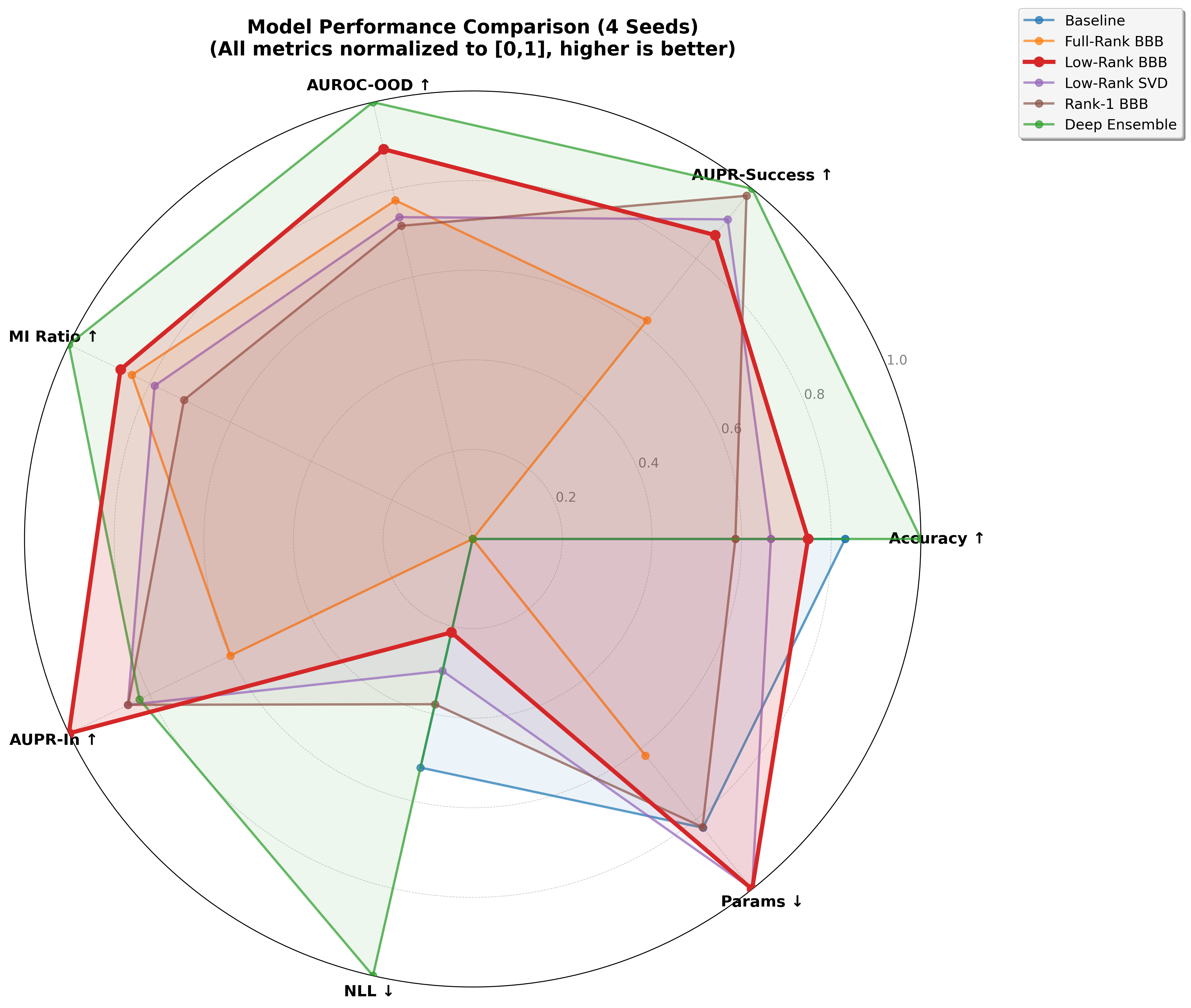
Best AUPR-In and second-best AUROC-OOD. Trains in 8.2 min vs 64.7 min for Deep Ensemble.

33× fewer params vs
Deep Ensemble
1.5M total params
full BNN
7.8× faster epoch vs
Deep Ensemble
Transformer radar 4 seeds

Aggregated uncertainty radar over 4 seeds — SST-2 Transformer.

SWAG comparison (appendix)

SWAG is a credible scalable posterior. It does not overturn the low-rank quality–efficiency tradeoff: on SST-2 it uses 208M parameters vs 1.47M; on MIMIC-III Low-Rank leads on MI-based OOD (0.802/0.788 vs 0.634/0.680).

SettingSWAG strengthLow-rank advantage
SST-2 Accuracy tied (0.808 vs 0.806) 1.47M params vs 208M; better AUPR-In
MIMIC-III Higher in-domain AUROC / NLL OOD MI: 0.802/0.788 vs 0.634/0.680
Beijing PM₂.₅ Higher raw coverage Narrower intervals; stronger OOD detection
09

Key insights

Calibration — OOD detection tradeoff

A consistent pattern across all three tasks: the rank constraint trades predictive sharpness (NLL) for broader epistemic uncertainty, benefiting OOD detection, abstention, and coverage.

MIMIC-III

Low-rank improves OOD detection despite weaker NLL than Deep Ensembles. Structured uncertainty outperforms under clinical domain shift.

SST-2

Deep Ensemble is stronger on NLL and OOD. Low-rank remains competitive at 33× fewer parameters — an entirely different efficiency regime.

Beijing PM₂.₅

Low-rank achieves best calibration, coverage, and selective prediction. OOD advantage is secondary to interval quality.

Hypothesis: The rank constraint on $\mathcal{R}_r$ enforces structured weight correlations (Lemma 3.2) that maintain broader epistemic uncertainty distributions. This benefits abstention, coverage, and OOD awareness at the cost of predictive sharpness. The tradeoff is task-dependent, with OOD-critical settings (e.g. clinical shift in MIMIC-III) favouring the low-rank posterior.

Result · Low-Rank Ensembling

Ensembling and low-rank are complementary — not competing.

Ensembling five low-rank members further improves every uncertainty metric, demonstrating that the two techniques stack. This opens a practical design space: smaller, cheaper ensembles of low-rank members can match or exceed a full-rank Deep Ensemble at a fraction of the parameter count.

0.638 → 0.731
+0.093
AUROC-OOD
0.166 → 0.054
−0.112
ECE ↓ (better)
0.523 → 0.415
−0.108
NLL ↓ (better)

Honest takeaway

The empirical message is not compression alone, and not that low-rank wins every metric.

Where low-rank shines

OOD separation on MIMIC; coverage and selective prediction on Beijing; efficiency-adjusted uncertainty on SST-2.

Where ensembles remain strong

In-distribution likelihood and predictive sharpness can favour Deep Ensembles. SWAG is a credible high-parameter baseline in some settings.

Why it matters

Trustworthy AI needs useful uncertainty under shift and deployment constraints, not only marginal NLL. SBNNs make that goal practical at scale.

10

Practical guidance

Four decisions govern how well SBNN works in practice. Here is what the paper's experiments teach about each.

1

Rank selection

Run ablation studies with reduced budget first — fewer epochs and fewer MC samples during validation. This is the primary method; no pretrained weights needed.

When a deterministic baseline already exists, use its singular value decay (SVD of trained weight matrices) as optional validation: rapid decay justifies the chosen rank. For SST-2, the embedding layer (70% of parameters) shows particularly fast decay.

Selected ranks in the paper: r=15 for MIMIC-III MLP, r=14/20 for Beijing LSTM, r=16 for SST-2 Transformer.

2

KL weight β and annealing

Start with β = 1/N_batches or β = 1/N_train. Higher β pushes the posterior toward the prior, improving OOD detection but degrading in-distribution NLL — tune based on which matters more for your task.

Always use KL annealing: ramp β from 0 to full over the first ~20 epochs. This lets the model find a good likelihood basin before the regularization penalty engages — especially important for LSTMs and Transformers where early KL dominance prevents learning entirely.

3

SVD initialization

Only use SVD warm-starting when a pretrained deterministic model already exists and comes for free. Results: modest gains on specific metrics (MIMIC AUROC: 0.898 vs 0.895; SST-2 AUPR-Succ: 0.923 vs 0.917), but inconsistent and task-dependent.

On Beijing LSTMs, random initialization outperforms SVD overall. The improvement does not justify training an additional deterministic model if one is not already available.

4

Architecture notes

All layers are drop-in Keras replacements — no other code changes needed. For LSTMs: forget gate bias = 1.0 and use weight caching (sample once per batch, reuse across time steps). For Transformers: the embedding layer alone is 70% of parameters; factorizing it with the sparsity trick gives the largest single efficiency gain.

At small scales (MLP, small LSTM), parameter reduction translates to memory savings, not wall-clock speedup — two matrix multiplications vs one. Efficiency gains emerge at transformer scale.

11

Additional evidence

Two supplementary experiments corroborate the main findings at small scale: a controlled MNIST study and a toy regression showing epistemic uncertainty behavior OOD.

MNIST: 19.5× compression, marginal calibration cost

4-layer MLP ($784 \to 1200 \to 1200 \to 10$, ReLU). Same scale-mixture prior. 50 MC samples at test time. Low-Rank uses $r=25$ for hidden layers. Low-Rank Laplace achieves the best NLL of all variants.

19.5× compression
4.79M → 245K
0.002 ECE gap vs
Full-Rank
97.3% accuracy
(vs 98.2% FR)

Calibration gap is only 0.002–0.0035 ECE in absolute terms across binning schemes — practically negligible for a 19.5× parameter reduction. Low-Rank Laplace achieves NLL 0.0607 vs 0.0795 for Full-Rank, suggesting heavier-tailed factor posteriors improve likelihood estimation.

Toy regression: conservative OOD uncertainty

MLP $1\to100\to100\to1$ (tanh). Train on $x\sim\text{Unif}[-0.1,\,0.6]$, evaluate on $x\in[-0.5,\,1.5]$. Low-Rank uses $r=16$ for the hidden layer — 65% fewer parameters.

2.01× OOD/in-domain
uncertainty ratio
1.90× same ratio
Full-Rank
65% parameter
reduction

Low-Rank maintains a wider absolute OOD uncertainty band (IQR 0.094 vs 0.048), providing more conservative credible intervals outside training support. The OOD/in-domain expansion ratio (2.01× vs 1.90×) confirms qualitative epistemic sensitivity is preserved — uncertainty grows when leaving the training domain, even in-domain uncertainty is higher, reflecting the rank constraint's regularizing effect.

12

Future directions

This work introduces SBNNs through the measure-theoretic singularity of the induced posterior. The singular posterior geometry provides both theoretical foundations and practical benefits for uncertainty quantification, making low-rank factorization a principled path toward scalable Bayesian deep learning. Several natural extensions open from here:

Adaptive rank selection

Ranks chosen by spectra, validation tradeoffs, or sparse priors (spike-and-slab) rather than fixed grids. Per-layer rank scheduling could further reduce parameter count.

Bayesian Transformers at scale

Extending to large language models and vision transformers. The $O(r(m+n))$ scaling makes this far more tractable than full-rank Bayesian inference.

Beyond Gaussian factors

Laplace, spike-and-slab, and richer factor distributions while keeping singular support. Non-Gaussian factors can represent multi-modal posterior landscapes.

Safety-critical deployment

Uncertainty that supports abstention, calibrated coverage, OOD awareness, and constrained deployment in clinical decision support and autonomous systems.

13

Resources

arXiv Paper abstract PDF Full paper GitHub Code and repositories Slides Interactive ICML presentation Homepage Main academic page

Citation

@inproceedings{toure2026singular,
  title     = {Singular Bayesian Neural Networks},
  author    = {Toure, Mame Diarra and Stephens, David A.},
  booktitle = {International Conference on Machine Learning},
  year      = {2026}
}